If you use Sony’s SXS cards or USB Hard Drives, Sony have a utility that allows you to check the status of your media and correctly format the media. This is particularly useful for reading the number of cycles your SXS card has reached.
The utility can also copy SXS cards to multiple destinations for simultaneous backups of your content. You can download the utility for free via the link below.
Sony’s Raw Viewer for raw and X-OCN file manipulation.
Sony’s raw viewer is an application that has just quietly rumbled away in the background. It’s never been a headline app, just one of those useful tools for viewing or transcoding Sony’s raw material. I’m quite sure that the majority of users of Sony’s raw material do their raw grading and processing in something other than raw viewer.
But this new version (2.3) really needs to be taken very seriously.
Better Quality Images.
For a start Sony have always had the best de-bayer algorithms for their raw content. If you de-bayer Sony raw in Resolve and compare it to the output from previous versions of Raw Viewer, the raw viewer content always looked just that little bit cleaner. The latest versions of Raw Viewer are even better as new and improved algorithms have been included! It might not render as fast, but it does look very nice and can certainly be worth using for any “problem” footage.
Class 480 XAVC and X-OCN.
Raw Viewer version 2.3 adds new export formats and support for Sony’s X-OCN files. You can now export to both XAVC class 480 and class 300, 10 or 12bit ProRes (HD only unfortunately), DPX and SStP. XAVC Class 480 is a new higher quality version of XAVC-I that could be used as a ProResHQ replacement in many instances.
Improved Image Processing.
Color grading is now easier than ever thanks to support for Tangent Wave tracker ball control panels along with new grading tools such as Tone Curve control. There is support for EDL’s and batch processing with all kind of process queue options allowing you to prioritise your renders. Although Raw Viewer doesn’t have the power of a full grading package it is very useful for dealing with problem shots as the higher quality de-bayer provides a cleaner image with fewer artefacts. You can always take advantage of this by transcoding from raw to 16 bit DPX or Open EXR so that the high quality de-bayer takes place in Raw Viewer and then do the actual grading in your chosen grading software.
HDR and Rec.2100
If you are producing HDR content version 2.3 also adds support for the PQ and HLG gamma curves and Rec.2100 It also now includes HDR waveform displays. You can use Raw Viewer to create HDR LUT’s too.
So all-in-all Raw Viewer has become a very powerful tool for Sony’s raw and XOCN content that can bring a noticeable improvement in image quality compared to de-bayering in many of the more commonly used grading packages.
If you are running the latest Mac Sierra OS the recent Pro Video Formats update, version 2.0.5 adds the ability to play back MXF OP1a files in Quick Time Player without the need to transcode.
Direct preview of an XAVC MXF file in the finder of OS Sierra.
You can also preview MXF files in the finder window directly! This is a big deal and very welcome, finally you don’t need special software to play back files wrapped in one of the most commonly used professional media wrappers. Of course you must have the codec installed on your computer, it won’t play a file you don’t have the codec for, but XAVC, ProRes and many other pro codecs are include in the update.
At the moment I am able to play back most MXF files including most XAVC and ProRes MXF’s. However some of my XAVC MXF’s are showing up as audio only files. I can still play back these files with 3rd party software, there is no change there. But for some reason I can’t play back every XAVC MXF file directly in Quicktime Player, so play as audio only. I’m not sure why some files are fine and others are not, but this is certainly a step in the right direction. Why it’s taken so long to make this possible I don’t really know, although I suspect it is now possible due to changes in the core Quicktime components of OS Sierra. You can apply this same Video Formats update to earlier OS’s but don’t gain the MXF playback.
I started writing this as an explanation of why I often choose not to use log for low light. But instead it’s ended up as an experiment you can try for yourself if you have a waveform monitor that will hopefully allow you to better understand the differences between log and standard gamma. Get a waveform display hooked up to your log camera and try this for yourself.
S-Log and other log gammas are wonderful things, but they are not the be-all and end-all of video gammas. They are designed for one specific purpose and that is to give cameras using conventional YCbCr or RGB recording methods the ability to record the greatest possible dynamic range with a limited amount of data, as a result there are some compromises made when using log. Unlike conventional gammas with a knee or gammas such as hypergammas and cinegammas, log gammas do not normally have any highlight roll off, but do have a shadow roll-off. Once you get above middle grey log gammas normally record every stop with almost exactly the same amount of data, right up to the clipping point where they hard clip. Below middle grey there is a roll off of data per stop as you go down towards the black clip point (as there is naturally less information in the shadows this is expected). So in many respects log gammas are almost the reverse of standard gammas. The highlight roll off that you may believe that you see with log is often just the natural way that real world highlights roll off anyway, after all there isn’t an infinite amount of light floating around (thank goodness). Or that apparent roll off is simply a display or LUT limitation.
An experiment for you to try.
Click on the chart to go to larger versions that you can download. Display it full screen on your computer and use it as a test chart. You may need to de-focus the camera slightly to avoid aliasing from the screens pixels.
If you have a waveform display and a grey scale chart you can actually see this behaviour. If you don’t have a chart use the grey scale posted here full screen on your computer monitor. Start with a conventional gamma, preferably REC-709. Point the camera at the chart and gradually open up the aperture. With normal gammas as you open the aperture you will see the steps between each grey bar open up and the steps spread apart until you reach the knee point, typically at 90% (assuming the knee is ON which is the default for most cameras). Once you hit the knee all those steps rapidly squash back together again.
What you are seeing on the waveform is conventional gamma behaviour where for each stop you go up in exposure you almost double the amount of data recorded, thus capturing the real world very accurately (although only within a limited range). Once you hit the knee everything is compressed together to increase the dynamic range using only a very small recording range, leaving the shadows and all important mid range well recorded. It’s this highlight compression that gives video the “video look”, washed out highlights with no contrast that look electronic.
If you repeat the same exercise with a hypergamma or cinegamma once again in the lower and mid range you will see the steps stretch apart on the waveform as you increase the exposure. But once you get to about 65-70% they stop stretching apart and now start to squeeze together. This is the highlight roll off of the hypergamma/cinegamma doing it’s thing. Once again compressing the highlights to get a greater dynamic range but doing this in a progressive gradual manner that tends to look much nicer than the hard knee. Even though this does look better than 709 + Knee in the vast majority of cases, we are still compressing the highlights, still throwing away a lot of data or highlight picture information that can never be recovered in post production no matter what you do.
Conventional video = Protect Your Highlights.
So in the conventional video world we are taught as cameramen to “protect the highlights”. Never overexpose because it looks bad and even grading won’t help a lot. If anything we will often err on the side of caution and expose a little low to avoid highlight issues. If you are using a Hypergamma or Cinegamma you really need to be careful with skin tones to keep them below that 65-70% beginning of the highlight roll off.
Now repeat the same experiment with Slog2 or S-log3. S-log2 is best for the experiment as it shows what is going on most clearly. Before you do it though mark middle grey on your waveform display with a piece of tape or similar. Middle grey for S-log2 is 32% (41% for S-log3).
Now open up the aperture and watch those steps between the grey scale bars. Below middle grey, as with the standard gammas you will see the gap between each bar open up. But take careful note of what happens above middle grey. Once you get above middle grey and all the way to the clip point the gap between each step remains the same.
So what’s happening now?
Well this is the S-log curve recording each stop above middle grey with the same amount of data. In addition there is NO highlight roll off. Even the very brightest step just below clipping will be same size as the one just above middle grey. In practice what this means is that it doesn’t make a great deal of difference where you expose for example skin tones, provided they are above middle grey and below clipping. After grading it will look more or less the same. In addition it means that that very brightest stop contains a lot of great, useable picture information. Compare that to Rec-709 or the Cinegammas/Hypergammas where the brightest stops are all squashed together and contain almost no contrast or picture information.
Now add in to the equation what is going on in the shadows. Log has less data in the shadows than standard gammas because you are recording a greater overall dynamic range, so each stop is recorded with overall less data.
Standard Gammas = More shadow data per stop, much less highlight data = Need to protect highlights.
Log= Less shadow data per stop, much more highlight data = Need to protect shadows.
Hopefully now you can see that with S-log we need to flip the way we shoot from protecting highlights to protecting shadows. When you shoot with conventional gammas most people expose so the mid range is OK, then take a look at the highlights to make sure they are not too bright and largely ignore whats going on in the shadows. With Log you need to do the opposite. Expose the mid range and then check the shadows to make sure they are not too dark. You can ignore the highlights.
Yes, thats’ right, when shooting log: IGNORE the highlights!
Cinegamma highlight roll off. Note how the tree branches in the highlights look strangled and ugly due to the lack of highlight data, hence “protect your highlights”.Graded S-Log2. Note how nice the same tree branches look because there is a lot of data in the highlights, but the shadows are a little crunchy. Hence: protect your shadows.
For a start you monitor or viewfinder isn’t going to be able to accurately reproduce the highlights as bright as they are . So typically they will look a lot more over exposed than they really are. In addition there is a ton of data in those highlights that you will be able to extract in the grade. But most importantly if you do underexpose your mid range will suffer, it will get noisy and your shadows will look terrible because there will be no data to work with.
When I shoot with log I always over expose by at least 1 stop above the manufacturer recommended levels. If you are using S-log2 or S-log3 that can be achieved by setting zebras to 70% and then checking that you are JUST starting to see zebras on something white in your shot such as a white shirt or piece of paper. If your camera has CineEI use an EI that is half of the cameras native ISO (I use 1000 or 800 EI for my FS7 or F5).
I hope these experiments with a grey scale and waveform help you understand what is going on with you gamma curves. One thing I will add is that while controlled over exposure is beneficial it can lead to some issues with grading. That’s because most LUT’s are designed for “correct” exposure so will typically look over exposed. Another issue is that if you simply reduce the gain level in post to compensate than the graded footage looks flat and washed out. This is because you are applying a linear correction to log footage. Fo a long tome I struggled to get pleasing results from over exposed log footage. The secret is to either use LUT’s that are offset to compensate for over exposure or to de-log the footage prior to grading using an S-Curve. I’ll cover both of these in a later article.
Chart showing S-Log2 and S-Log3 plotted against f-stops and code values.
What about shooting in low light?
OK, now lets imagine we are shooting a dark or low light scene. It’s dark enough that even if we open the aperture all the way the brightest parts of the scene (ignoring things like street lights) do not reach clipping (92% with S-Log3 or 109% with S-Log2). This means two things. 1: The scene has a dynamic range less than 14 stops and 2: We are not utilising all of the recording data available to us. We are wasting data.
Log exposed so that the scene fills the entire curve puts around 100 code values (or luma shades) per stop above middle grey for S-log2 and 75 code values for S-Log3 with a 10 bit codec. If your codec is only 8 bit then that becomes 25 for S-log2 and 19 code values for S-Log3. And that’s ONLY if you are recording a signal that fills the full range from black clip to white clip.
3 stops below middle grey there is very little data, about thirty 10 bit code values for S-Log2 and about 45 for S-log3. Once again if the codec is 8 bit you have much less, about 7 for S-Log2 and about 11 for S-log2. As a result the darker parts of your recorded scene will be recorded with very little data and very few shades. This impacts how much you can grade the image in post as there is very little picture information in the darker parts of the shot and noise tends to look quite coarse as it is only recorded with a limited number of steps or levels (this is particularly true of 8 bit codecs and an area where 8 bit recordings can be problematic).
So what happens if we use a standard gamma curve?
Lets say we now shoot the same scene with a standard gamma curve, perhaps REC-709. One point to note with Sony cameras like the FS5, FS7, F5/F55 etc is that the standard gammas normally have a native ISO one to two stops lower than S-Log. That’s because the standard gammas ignore the darkest couple of stops that are recorded when in log. After all there is very little really useable picture information down there in all the noise.
Now our limited dynamic range scene will be filling much more of our recording range. So straight away we have more data per stop because we are utilising a bigger portion of the recording range. In addition because our recorded levels will be higher in our recording range there will be more data per stop, typically double the data especially in the darker parts of the recorded image. This means than any noise is recorded more accurately which results in smoother looking noise. It also means there is more data available for any post production manipulation.
But what about those dark scenes with problem highlights such as street lights?
This an area where Cinegammas or Hypergammas are very useful. The problem highlights like strret lights normally only make up a very small part of your your overall scene. So unless you are shooting for HDR display it’s a huge waste to use S-log just to bring some highlights into range as you make big compromises to the rest of the image and you’ll never be able to show them accurately in the finished image anyway as they will exceed the dynamic range of the TV display. Instead for these situations a Hypergamma or Cinegamma works well because below about 70% exposure Hypergammas and cinegammas are very similar to Rec-709 so you will have lots of data in the shadows and mid range where you really need it. The highlights will be up in the highlight roll off area where the data levels or number of recorded shades are rolled off. So the highlights still get recorded, perhaps without clipping, but you are only giving away a small amount of data to do this. The highlights possibly won’t look quite as nice as if recorded with log, but they are typically only a small part of the scene and the rest of the scene especially the shadows and mid tones will end up looking much better as the noise will be smoother and there will be more data in that all important mid-range.
This comes up a lot. People shoot in log, take it in to the grading suite or worse still the edit suite, try to grade it and are less than happy with the end result. Some people really struggle to make log look good.
Why is this? Well we normally view our footage on a TV, monitor or computer screen that uses a gamma curve that follows what is known as a “power law” curve. While this isn’t actually a true linear type of curve, it most certainly is not a log curve. Rec-709 is a “power law” curve.
The key thing about this when trying to understand why log can be tricky to grade is that in the real world, the world that we see, as you go up in brightness for each stop brighter you go, there is twice as much light. A power law gamma such as 709 follows this fairly closely as each brighter stop recorded uses a lot more data than the previous. But log is quite different, to save space, log uses more or less the same amount of data for each stop, with the exception of the darkest stops that have very little data anyway. So conventional gamma = much more data per brighter stop, log gamma = same data for each stop.
So time to sit down somewhere quiet before trying to follow this crude explanation. It’s not totally scientifically accurate, but I hope you will get the point and I hope you will see why trying to grade Log in a conventional edit suite might not be the best thing to try to do.
Lets consider a scene where the brightness might be represented by some values and we record this scene with a convention gamma curve. The values recorded might go something like this, each additional stop being double the previous:
CONVENTIONAL RECORDING: 1 – 2 – 4 – 8 – 16
Then in post production we decide it’s a bit dark so we increase the gain by a factor of two to make the image brighter, the output becomes:
CONVENTIONAL AFTER 2x GAIN: 2 – 4 – 8 – 16 – 32
Notice that the number sequence uses the same numbers but they get bigger, doubling for each stop. In an image this would equate to a brighter picture with the same contrast.
Now lets consider recording in log. Log uses the same amount of data per stop, so the recorded levels for exactly the same scene would be something like this:
LOG RECORDING (“2” for each stop): 1 – 2 – 4 – 6 – 8.
If in post production if we add a factor of two gain adjustment we will get the same brightness as our uncorrected conventional recording, both reach 16, but look at the middle numbers they are different, the CONTRAST will be different.
LOG AFTER 2x GAIN: 2 – 4 – 8 – 12 – 16.
It gets even worse if we want to make the log footage as bright as the corrected conventional footage. To make the log image equally bright to the corrected conventional footage we have to use 4x gain. Then we get:
LOG AFTER 4x GAIN: 4 – 8 – 16 – 24 – 32
So now we have the same final brightness for both the corrected conventional and corrected log footage but the contrast is very different. The darks and mids from the log have become brighter than they should be, compare this to the conventional after 2x gain. The contrast has changed. This is the problem with log. Applying simple gain adjustments to log footage results in both a contrast and brightness change.
So when grading log footage you will typically need to make separate corrections to the low middle and high range. You want a lift control to adjust the blacks and deep shadows, a mid point level shift for the mid range and a high end level shift. You don’t want to use gain as not only will it make the picture brighter and darker but it will also make it more or less contrasty.
One way to grade log is to use a curve tool to alter the shape of the gamma curve, pulling down the blacks while stretching out the whites. In DaVinci Resolve you have a set of log grading color wheels as well as the conventional primary color wheels. Another way to grade log is to apply a LUT to it and then grade in more conventional 709 space, although arguably any grading is best done prior to the LUT.
Possibly the best way is to use ACES. The Academy of Motion Pictures workflow takes your footage, whether log or linear and converts it to true linear within the software. Then all corrections take place in linear space where it is much more intuitive before finally be output from ACES with a film curve applied.
I’ve been running a lot of workshops recently looking at creating LUT’s and scene files for the FS7, F5 and F55. One interesting observation is that when creating a stylised look, almost always the way the footage looks before you grade can have a very big impact on who far you are prepared to push your grade to create a stylised look.
What do I mean by this? Well if you start off in your grading suite looking at some nicely exposed footage with accurate color and a realistic representation of the original scene, when you start to push and pull the colors in the image the pictures start to look a little “wrong” and this might restrict how far you are prepared to push things as it goes against human nature to make things look wrong.
If on the other hand you were to bring all your footage in to the grading suite with a highly stylised look straight from the camera, because it’s already unlike the real world, you are probably going to be more inclined to further stylise the look as you have never seen the material accurately represent the real world so don’t notice that it doesn’t look “right”.
An interesting test to try is to bring in some footage into the grade and apply a very stylised look via a LUT and then grade the footage. Try to avoid viewing the footage with a vanilla true to life LUT if you can.
Then bring in the same or similar footage with a vanilla true to life LUT and see how far you are prepared to push the material before you star getting concerned that it no longer looks right. You will probably find that you will push the stylised footage further than the normal looking material.
As another example if you take almost any recent blockbuster movie and start to analyse the look of the images you will find that most use a very narrow palette of orange skin tones along with blue/green and teal. Imagine what you would think if your TV news was graded this way, I’m sure most people would think that the camera was broken. If a movie was to intercut the stylised “look” images with nicely exposed, naturally colored images I think the stylised images would be the ones that most people would find objectionable as they just wouldn’t look right. But when you watch a movie and everything has the same coherent stylised look it works and it can look really great.
In my workshops when I introduce some of my film style LUT’s for the first time (after looking at normal images), sometimes people really don’t like them as they look wrong. The colors are off, it’s all a bit blue, it’s too contrasty, are all common comments. But if you show someone a video that uses the same stylised look throughout the film then most people like the look. So when assessing a look or style try to look at it in the right context and try to look at it without seeing a “normal” picture. I find it helps to go and make a coffee between viewing the normal footage and then viewing the same material with a stylised look.
Another thing that happens is the longer you view a stylised look the more “normal” it becomes as your brain adapts to the new look.
In fact while typing this I have the TV on. In the commercial break that’s just been on most of the ads used a natural color palette. Then one ad came on that used a film style palette (orange/teal). The film style palette looked really, really odd in the middle of the normal looking ads. But on it’s own that ad does have a very film like quality too it. It’s just that when surrounded by normal looking footage it really stands out and as a result looks wrong.
I have some more LUT’s to share in the coming days, so check back soon for some film like LUT’s for the FS7/F5/F55 and A7s.
I had the pleasure of listening to Pablo Garcia Soriano the resident DiT/Colorist at the Sony Digital Motion Picture Center at Pinewood Studios last week talk about grading modern digital cinema video cameras during the WTS event .
The thrust of his talk was about exposure and how getting the exposure right during the shoot makes a huge difference in how much you can grade the footage in post. His main observation was that many people are under exposing the camera and this leads to excessive noise which makes the pictures hard to grade.
There isn’t really any real way to reduce the noise in a video camera because nothing you normally do can change the sensitivity of the sensor or the amount of noise it produces. Sure, noise reduction can mask noise, but it doesn’t really get rid of it and it often introduces other artefacts. So the only way to change the all important signal to noise ratio, if you can’t change the noise, is to change the signal.
In a video camera that means opening the aperture and letting in more light. More light means a bigger video signal and as the noise remains more or less constant that means a better signal to noise ratio.
If you are shooting log or raw then you do have a fair amount of leeway with your exposure. You can’t go completely crazy with log, but you can often over expose by a stop or two with no major issues. You know, I really don’t like using the term “over-expose” in these situations. But that’s what you might want to do, to let in up to 2 stops more light than you would normally.
In photography, photographers shooting raw have been using a technique called exposing to the right (ETTR) for a long time. The term comes from the use of a histogram to gauge exposure and then exposing so the the signal goes as far to the right on the histogram as possible (the right being the “bright” side of the scale). If you really wanted to have the best possible signal to noise ratio you could use this method for video too. But ETTR means setting your exposure based on your brightest highlights and as highlights will be different from shot to shot this means the mid range of you shot will go up and down in exposure depending on how bright the highlights are. This is a nightmare for the colorist as it’s the mid-tones and mid range that is the most important, this is what the viewer notices more than anything else. If these are all over the place the colorist has to work very hard to normalise the levels and it can lead to a lot of variability in the footage. So while ETTR might be the best way to get the very best signal to noise ratio (SNR), you still need to be consistent from shot to shot so really you need to expose for mid range consistency, but shift that mid range a little brighter to get a better SNR.
Pablo told his audience that just about any modern digital cinema camera will happily tolerate at least 3/4 of a stop of over exposure and he would always prefer footage with very slightly clipped highlights rather than deep shadows lost in the noise. He showed a lovely example of a dark red car that was “correctly” exposed. The deep red body panels of the car were full of noise and this made grading the shot really tough even though it had been exposed by the book.
When I shoot with my F5 or FS7 I always rate them a stop slower that the native ISO of 2000. So I set my EI to 1000 or even 800 and this gives me great results. With the F55 I rate that at 800 or even 640EI. The F65 at 400EI.
If you ever get offered a chance to see one of Pablo’s demos at the DMPCE go and have a listen. He’s very good.
What do we really mean when we talk about exposure?
If you come from a film background you will know that exposure is the measure of how much light is allowed to fall on the film. This is controlled by two things, the shutter speed and the aperture of the lens. How you set these is determined by how sensitive the film stock is to light.
But what about in the video world? Well exposure means exactly the same thing, it’s how much light we allow our video sensor to capture. Controlled by shutter speed and aperture. The amount of light we need to allow to fall on the sensor is dependant on the sensitivity of the sensor, much like film. But with video there is another variable and that is the gamma curve…. or is it????
This is an area where a lot of video camera operators have trouble, especially when you start dealing with more exotic gamma curves such as log. The reason for the problem is down to the fact that most video camera operators are taught or have learnt to expose their footage at specific video levels. For example if you’re shooting for TV it’s quite normal to shoot so that white is around 90%, skin tones are around 70% and middle grey is in the middle, somewhere around the 45% mark. And that’s been the way it’s been done for decades. It’s certainly how I was taught to expose a video camera.
If you have a video camera with different gamma curves try a simple test. Set the camera to its standard TV gamma (rec-709 or similar). Expose the shot so that it looks right, then change the gamma curve without changing the aperture or shutter speed. What happens? Well the pictures will get brighter or darker, there will be brightness differences between the different gamma curves. This isn’t an exposure change, after all you haven’t changed the amount of light falling on the sensor, this is a change in the gamma curve and the values at which it records different brightnesses.
An example of this would be setting a camera to Rec-709 and exposing white at 90% then switching to S-log3 (keeping the same ISO for both) and white would drop down to 61%. The exposure hasn’t changed, just the recording levels.
It’s really important to understand that different gammas are supposed to have different recording levels. Rec-709 has a 6 stop dynamic range (without adding a knee). So between 0% and around 100% we fit 6 stops with white falling at 85-90%. So if we want to record 14 stops where do we fit in the extra 8 stops that S-Log3 offers when we are already using 0 to 100% for 6 stops with 709?? The answer is we shift the range. By putting the 6 stops that 709 can record between around 15% and 68% with white falling at 61% we make room above and below the original 709 range to fit in another 8 stops.
So a difference in image brightness when changing gamma curves does not represent a change in exposure, it represents a change in recording range. The only way to really change the exposure is to change the aperture and shutter speed. It’s really, really important to understand this.
Furthermore your exposure will only ever look visibly correct when the gamma curve of the display device is the same as the capture gamma curve. So if shooting log and viewing on a normal TV or viewfinder that typically has 709 gamma the picture will not look right. So not only are the levels different to those we have become used to with traditional video but the picture looks wrong too.
As more and more exotic (or at least non-standard) gamma curves become common place it’s very important that we learn to think about what exposure really is. It isn’t how bright the image is (although this is related to exposure) it is about letting the appropriate amount of light fall on the sensor. How do we determine the correct amount of light? Well we need to measure it using a waveform scope, zebras etc, BUT you must also know the correct reference levels for the gamma you are using for a white or middle grey target.
When you want two cameras to have matching timecode you need to synchronise not just the time code but also the frame rates of both cameras. Remember timecode is a counter that counts the frames the camera is recording. If one camera is recording more frames than the other, then even with a timecode cable between both cameras the timecode will drift during long takes. So for perfect timecode sync you must also ensure the frame rates of both cameras is also identical by using Genlock to synchronise the frame rates.
Genlock is only going to make a difference if it is always kept connected. As soon as you disconnect the Genlock the cameras will start to drift. If using genlock first connect the Ref output to the Genlock in. Then while this is still connected connect the TC out to TC in. Both cameras should be set to Free-run timecode with the TC on the master camera set to the time of day or whatever time you wish both cameras to have. If you are not going to keep the genlock cable connected for the duration of the shoot, then don’t bother with it at all, as it will make no difference just connecting it for a few minutes while you sync the TC.
In the case of a Sony camera when the TC out is connected to the TC in of the slave camera, the slave camera will normally display EXT-LK when the timecode signals are locked.
Genlock: Synchronises the precise timing of the frame rates of the cameras. So taking a reference out from one camera and feeding it to the Genlock input of another will cause both cameras to run precisely in sync while the two cameras are still connected together. While connected by genlock the frame counts of both camera (and the timecode counts) will remain in sync. As soon as you remove the genlock sync cable the cameras will start to drift apart. The amount of sync (and timecode) drift will depend on many factors, but with a Sony camera will most likely be in the order of a at least a few seconds a day, sometimes as much as a few minutes.
Timecode: Connecting the TC out of one camera to the TC in of another will cause the time code in the receiving camera to sync to the nearest possible frame number of the sending camera when the receiving camera is set to free run while the camera is in standby. When the TC is disconnected both cameras timecode will continue to count according to the frame rate that the camera is running at. If the cameras are genlocked, then as the frame sync and frame count is the same then so too will be the timecode counts. If the cameras are not genlocked then the timecode counts will drift by the same amount as the sync drift.
Timecode sync only and long takes can be problematic. If the timecodes of two cameras are jam sync’d but there is no genlock then on long takes timecode drift may be apparent. When you press the record button the timecodes of both cameras will normally be in sync, forced into sync by the timecode signal. But when the cameras are rolling the timecode will count the actual frames recorded and ignor the timecode input. So if the cameras are not synchronised via genlock then they may not be in true sync so one camera may be running fractionally faster than the other and as a result in long clips there may be timecode differences as one camera records more frames than the other in the same time period.
This is not going to be a tutorial on editing or grading. Just an outline guide on how to work with S-log2, mainly with Adobe Premiere and DaVinci Resolve. These are the software packages that I use. Once upon a time I was an FCP user, but I have never been able to get on with FCP-X. So I switched to Premiere CC which now offers some of the widest and best codec support as well as an editing interface very similar to FCP. For grading I like DaVinci Resolve. It’s very powerful and simple to use, plus the Lite version is completely free. If you download Resolve it comes with a very good tutorial. Follow that tutorial and you’ll be editing and grading with Resolve in just a few hours.
The first thing to remember about S-Log2/S-gamut material is that it has a different gamma and colour space used by almost every TV and monitor in use today. So to get pictures that look right on a TV we will need to convert the S-Log2 to the standard used by normal HD TV’s which is know as Rec-709. The best way to do this is via a Look Up Table or LUT.
Don’t be afraid of LUT’s. It might be a new concept for you, but really LUT’s are easy to use and when used right they bring many benefits. Many people like myself share LUT’s online, so do a google search and you will find many different looks and styles that you can download for your project.
So what is a LUT? It’s a simple table of values that converts one set of signal levels to another. You may come across different types of LUT’s… 1D, 3D, Cube etc. At a basic level these all do the same thing, there are some differences but at this stage we don’t need to worry about those differences. For grading and post production correction, in the vast majority of cases you will want to use a 3D Cube LUT. This is the most common type of LUT. The LUT’s that you use must be designed for the gamma curve and colour space that the material was shot in and the gamma curve and colorspace you want to end up in. So, in the case of a Sony camera, be that an A7s, A7r, A6300 or whatever we want LUT’s that are designed for either S-Log2 and S-Gamut or S-Log3 and SGamut3.cine. LUT’s designed for anything other than this will still transform the footage, but the end results will be unpredictable as the tables input values will not match the correct values for S-Log2/S-Log3.
One of the nice things about LUT’s is that they are non-destructive. That is to say that if you add a LUT to a clip you are not actually changing the original clip, you are simply altering the way the clip is displayed. If you don’t like the way the clip looks you can just try a different LUT.
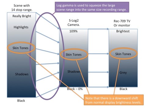
If you followed the A7s shooting guide then you will remember that S-Log2 or S-Log3 takes a very large shooting scene dynamic range (14 stops) and squeezes that down to fit in a standard video camera recording range. When this squeezed or compressed together range is then shown on a conventional REC-709 TV with a relatively small dynamic range (6 stops) the end result is a flat looking, low contrast image where the overall levels are shifted down a bit, so as well as being low contrast and flat the pictures may also look dark.
To make room for the extra dynamic range and the ability to record very bright objects, white and mid tones are shifted down in level.The on screen contrast appears reduced as the capture contrast is greater than the display contrast.
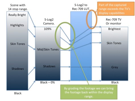
To make the pictures on our conventional 709 TV or computer moniotr have a normal contrast range, in post production we need to expand the the squeezed recorded S-Log2/S-Log3 range to the display range of REC-709. To do this we apply an S-Log2 or S-Log3 to Rec-709 LUT to the footage during the post production process. The LUT table will shift the S-log input values to the correct REC-709 output values. This can be done either with your edit software or dedicated grading software. But, we may need to do more than just add the LUT.
Adding a LUT in post production expands the squeezed S-Log2 recording back to a normal contrast range.
There is a problem because normal TV’s only have a limited display range, often smaller that the recorded image range. So when we expand the squeezed S-Log2/S-Log3 footage back to a normal contrast range the amount of dynamic range in the recording exceeds the dynamic range that the TV can display so the highlights and brighter parts of the picture are lost, they are no longer seen and as a result the footage may now look over exposed.
With the dynamic range now expanded by the LUT the recordings brightness range exceeds the range that the TV or monitor can show, so while the contrast is correct, the pictures may look over exposed.
But don’t panic! The brightness information is still there in your footage, it hasn’t been lost, it just can’t be displayed. So we need to tweak and fine tune the footage to bring the brighter parts of the image back in to range. This is typivally called “grading” or color correcting the material.
Normally you want to grade the clip before it passes through the LUT as prior to the LUT the full range of the footage is always retained. The normal procedure is to add the LUT to the clip or footage as an output LUT, that is to say the LUT is on the output from the grading system. Although it’s preferable to have the LUT after any corrections, don’t worry too much about where your LUT goes. Most edit and grading software will still retain the full range of everything you have recorded, even if you can’t always see it on the TV or monitor.
By grading or adjusting the footage before it enters the LUT we can bring the highlights back within the range that the TV or monitor can show.
If you chose to deliberately over expose the camera by a stop or two to get the best from the 8 bit recordings (see part one of the guide) then the LUT that you should use should also incorporate compensation for this over exposure. The LUT sets that I have provided for the Sony Alpha cameras includes LUTs that have compensation for +1 and +2 stops of over exposure.
IN PRACTICE.
So how do we do this in practice?
First of all you need some LUT’s. If you haven’t already downloaded my LUT’s please download one or both of my LUT sets:
To start off with you can just edit your S-Log footage as you would normally. Don’t worry too much about adding a LUT at the edit stage. Once the edit is locked down you have two choices. You can either export your edit to a dedicated grading package, or, if your edit package supports LUT’s you can add the LUT’s directly in the edit application.
In Premiere CC you use the built in Lumetri filter plugin found under the “filters”, “color correction filters” tab (not the Lumetri Looks).
In all the above cases you add the filter or plugin to the clip and then select the LUT that you wish to use. It really is very easy. Once you have applied the LUT you can then further fine tune and adjust the clip using the normal color correction tools. To apply the same LUT to multiple clips simply select a clip that already has the LUT applied and hit “copy” or “control C” and then select the other clips that you wish to apply the LUT to and then select “paste – attributes” to copy the filter settings to the other clips.
Exporting Your Project To Resolve (or another grading package).
This is my preferred method for grading as you will normally find that you have much better correction tools in a dedicated grading package. What you don’t want to do is to render out your edit project and then take that render into the grading package. What you really want to do is export an edit list or XML file that contains the details of your project. The you open that edit list or XML file in the grading package. This should then open the original source clips as an edited timeline that matches the timeline you have in your edit software so that you can work directly with the original material. Again you would just edit as normal in your edit application and then export the project or sequence as preferably an XML file or a CMX EDL. XML is preferred and has the best compatibility with other applications.
Once you have imported the project into the grading package you then want to apply your chosen LUT. If you are using the same LUT for the entire project then the LUT can be added as an “Output” LUT for the entire project. In this way the LUT acts on the output of your project as a final global LUT. Any grading that you do will then happen prior to the LUT which is the best way to do things. If you want to apply different LUT’s to different clips then you can add a LUT to individual clips. If the grading application uses nodes then the LUT should be on the last node so that any grading takes place in nodes prior to the LUT.
Once you have added your LUT’s and graded your footage you have a couple of choices. You can normally either render out a single clip that is a compilation of all the clips in the edit or you can render the graded footage out as individual clips. I normally render out individual clips with the same file names as the original source clips, just saved in a different folder. This way I can return to my edit software and swap the original clips for the rendered and graded clips in the same project. Doing this allows me to make changes to the edit or add captions and effects that may not be possible to add in the grading software.
This website uses cookies to improve your experience. We'll assume you're ok with this, but you can opt-out if you wish. Read More
Necessary cookies help make a website usable by enabling basic functions like page navigation and access to secure areas of the website. The website cannot function properly without these cookies.
Name
Domain
Purpose
Expiry
Type
wpl_user_preference
www.xdcam-user.com
WP GDPR Cookie Consent Preferences
1 year
HTTP
YSC
youtube.com
YouTube session cookie.
54 years
HTTP
Marketing cookies are used to track visitors across websites. The intention is to display ads that are relevant and engaging for the individual user and thereby more valuable for publishers and third party advertisers.
Name
Domain
Purpose
Expiry
Type
VISITOR_INFO1_LIVE
youtube.com
YouTube cookie.
6 months
HTTP
Analytics cookies help website owners to understand how visitors interact with websites by collecting and reporting information anonymously.
Name
Domain
Purpose
Expiry
Type
__utma
xdcam-user.com
Google Analytics long-term user and session tracking identifier.
2 years
HTTP
__utmc
xdcam-user.com
Legacy Google Analytics short-term technical cookie used along with __utmb to determine new users sessions.
54 years
HTTP
__utmz
xdcam-user.com
Google Analytics campaign and traffic source tracking cookie.
6 months
HTTP
__utmt
xdcam-user.com
Google Analytics technical cookie used to throttle request rate.
Session
HTTP
__utmb
xdcam-user.com
Google Analytics short-term functional cookie used to determine new users and sessions.
Session
HTTP
Preference cookies enable a website to remember information that changes the way the website behaves or looks, like your preferred language or the region that you are in.
Name
Domain
Purpose
Expiry
Type
__cf_bm
onesignal.com
Generic CloudFlare functional cookie.
Session
HTTP
NID
translate-pa.googleapis.com
Google unique id for preferences.
6 months
HTTP
Unclassified cookies are cookies that we are in the process of classifying, together with the providers of individual cookies.
Name
Domain
Purpose
Expiry
Type
_ir
api.pinterest.com
---
Session
---
Cookies are small text files that can be used by websites to make a user's experience more efficient. The law states that we can store cookies on your device if they are strictly necessary for the operation of this site. For all other types of cookies we need your permission. This site uses different types of cookies. Some cookies are placed by third party services that appear on our pages.